This is the third in a series of articles, collaboratively written by data and solution architects at Myers-Holum, Inc., PRA Health Sciences, and Google, describing an architectural framework for conversions of data warehouses from Teradata to the Google Cloud Platform.  The series will explore common architectural patterns for Teradata data warehouses and outline best-practice guidelines for porting these patterns to the GCP toolset.

David Chu, Knute Holum and Darius Kemeklis, Myers-Holum, Inc.

Michael Trolier, Ph.D., PRA Health Sciences

August 2018

Table of Contents

⇒ Capture versus land

⇒ What does a data warehouse look like on Google Cloud Platform?

⇒ Dust-off Your Semantic Model

⇒ Creating the Physical Schema

⇒ Example using our Travel Reservation Model

⇒ Semantic Model Example using our Travel Reservation Star Schema

⇒ Physical Model Example for Reservation_Payment_Fact

⇒ Physical Model Example for Room_Reservation_Fact

⇒ Additional Considerations

⇒ Wrap-up, what’s next

Recap:  In the first article of this series, “Article 1: Understanding Your Current Data Warehouse”, we discussed source data capture as the first architectural layer of most data warehouses.  We categorized the three types of source capture processes (pull, push or stream) and the typical Teradata implementation strategies for landing the data into the data warehouse for each type of process.

In the second article of this series, “Article 2: Source Data Capture”, we recommended the creation of a unified landing model, as an architectural component we called the “Landing Zone”.  All source data capture activities target the Landing Zone with associated control processes managing the accessibility and lifespan of those slices of captured data.   We discussed the detailed requirements you should consider in your implementation of the Landing Zone to facilitate your decisions on whether existing Teradata source data capture processes can truly be converted.

Conversion versus Re-implementation:  As you read this series of articles, we are going to differentiate between approaches for converting your data warehouse from Teradata to the Google Cloud Platform versus re-implementing your data warehouse in Google Cloud Platform.  Arbitrarily, we are going to assume certain differences between the two approaches.   The conversion project will be assumed as justified based on an expense reduction/capital spend avoidance ROI model, and therefore the cost of the conversion must be constrained to fit within this cost reduction model.   We would also expect the implementation timeline to be oriented toward a single deliverable, and timed such that the next Teradata infrastructure upgrade can be avoided.

On the other hand, the reimplementation project will be assumed as justified based on a business benefit model, with implementation (capital) costs factored into the internal rate of return for the project.  We would also expect the implementation timeline to be phased into multiple deliverables based on the order of business initiatives you want to undertake.

⇒ What does a data warehouse look like on Google Cloud Platform?

To understand the scope of your Teradata conversion effort, you need to understand both the source and target requirements.  Only with this knowledge, can you understand the data integration processes in between that will make up the bulk of your conversion effort.

Cloud BigQuery is Google’s recommended technology for implementing your data warehouse.   BigQuery is a fully managed, petabyte-scale, low-cost enterprise data warehouse for business intelligence.  It is probably one of the principal reasons you are considering a data warehouse conversion.  

Migrating your Teradata data warehouse means that you will be instantiating your semantic logical data model into a new physical data model optimized for BigQuery.  As you recall in Article 1, we discussed the importance understanding how the Teradata semantic layer has been implemented and the extent to which it is actually being used.    

The migration from Teradata will require a bottom up approach, you will be implementing a series of BigQuery tables representing the semantic requirements of a given subject area.  Subject areas will be integrated using common dimensional data (such as customer, product, supplier, organization or employee).

The bottom up approach will allow for an iterative conversion process.  Subject areas can be implemented using an incremental approach, where you weigh subject areas that provide highest conversion benefit.  For example, at our client “Company X”, the customer marketing subject area consumes 60 percent of the existing Teradata storage capacity.  In addition, 14 of the top 25 most frequently used queries access this data.  Therefore, migrating this subject area off Teradata not only provides BigQuery benefits to the users of customer marketing, but also to the remaining Teradata users utilizing different subject areas which now benefit from the new Teradata capacity now available.  

⇒ Dust-off Your Semantic Model

You will need a semantic logical data model that represents the data presentation requirements for a given subject area before you can begin any BigQuery physical design.  We recommend using a star schema (following Kimball standards) as the basis for your semantic model.  We also recommend the use of a data modeling tool (ER/Studio, CA-ERWin, InfoSphere, etc.) to maintain it.   The metadata created and maintained in the data modeling tool will become an important component of your overall data warehouse metadata strategy, which we will cover in a future article.    

If you do not have an existing semantic logical data model, creating one in a conversion scenario is not that difficult.  Remember you have an existing Teradata implementation you can analyze to create it.   Here are some approaches for doing that:

• Use your Teradata database views:
  • If you have used views to standardize end user access to your data warehouse, and those views are more than simple wrappers of your data warehouse tables, then these views may be an effective approach for creating a semantic logical data model.
• Use the semantic model from your BI tool:
  • Many BI products like Business Objects, MicroStrategy, and Cognos incorporate semantic layers.
  • If you have predominantly standardized end user access via the BI tool, this may be an effective source for creating a semantic logical data model.
• Analyze your current reports and dashboards:
  • Within a representative sample of reports:
    • What is the underlying granularity of the report (fact level)
    • To what level is the report aggregated (by region, by fiscal period, by product)
    • What other dimensional data is reported
  • We create an Excel spreadsheet to contain this analysis with the rows reflecting the underlying granularity and the columns reflecting the aggregate levels and other dimensions.

⇒ Creating the Star Schema

As you create the star schema representing your semantic model, it is important to focus on the following objectives:

• Identifying fact tables and declaring their associated grain:
  • Fact tables tend to mirror business processes and the associated measures for that business process.  It is important that you use this information to declare the grain of the fact table independently of the levels of granularity contained within the source data.  For example, our sample reservation source model contains levels of granularity reflecting the reservation (order level), reservation item (order item level), booking level (inventory level) and booking detail (pricing level).   However, our reservation star schema contains fact tables representing the business processes at the grain we want to analyze: reservation, reservation item, and reservation payment.  What you name your fact tables should clearly indicate the grain.  
  • Fact tables always have a date (or date/time) dimension, typically representing the transaction or event date.  And that date dimension is typically qualified each time the fact table is accessed by an end user.  In other words, we are looking in advance to identify how we intend to the date partition each fact table.
  • Fact tables are the only tables in a star schema with a composite primary key.  That primary key is always composed of the date dimension and enough other referenced dimensions to guarantee uniqueness.    
• Identifying the dimension types (type 1, 2 or 3):
  • As you identify the dimensions that apply to each fact table, you need to understand the strategy to handle any change in the associated dimensional values.  Thus the dimension should be clearly declared as to its type; where type 1 means overwrite the value, type 2 means add a dimensional row, and type 3 means add a dimensional column.  
  • In effect, the type of dimension consistently declares the point in time relationship between the dimensional values and the associated fact measures.   Having a consistent definition of this point in time relationship will be immensely helpful as when we create the physical schema, and further physically de-normalize it for performance.
  • For type 2 and type 3 dimensions, don’t automatically assume an effective end date (or current indicator) is needed.   It has no relationship to the associated fact table and typically is not mandatory as a dimension attribute.   In the next article, we will identify the significant data integration benefit of not having to maintain it.  
  • Remember it is OK to have the same dimension as both type 1 and type 2.  This gives you both the historical and as the current point in time in relation to the fact.  You would simply define the same dimension as different entities in your logical model.          
• Identifying aggregate needs:
  • Make sure you have the dimensions available to support the common aggregations you captured during your analysis of your current reports and dashboards.   If you have implemented aggregate awareness via either Teradata join indexes or within your BI tool, this will be another method of identifying these dimensions you summarize by.
  • Since BigQuery is column oriented store and can very efficiently aggregate column values, we typically do not model pre-computed aggregates (aka summary tables).      

⇒ Creating the Physical Schema

The physical schema represents how your end users and associated end user oriented tool sets will see the data warehouse in BigQuery.  Implementing this schema requires the same compromise between ease of use (with potentially inefficient access) versus efficient data access (with potential difficulty to use) that we have all made many times before.  Our physical design approach seeks to optimize ease of use for as many business use cases as possible but also recognizing that physical schema optimization for query performance and cost may be needed in certain situations.

BigQuery’s ability to support a huge data set is a clear advantage of the Google product and most of our clients have at least future plans to utilize this capability.  However, it is important to realize that in a conversion scenario, typical data set sizes coming from Teradata will allow a degree of sub-optimal design while still meeting expected end user SLA’s and cost constraints.  

BigQuery physical schema optimization revolves around two key capabilities:

• Implementing date based partitioning
• Using nested and repeating fields to flatten multiple tables into one table to co-locate the data and eliminate required joins

Our design approach seeks to apply a consistent set of physical modeling rules to the star schema logical model, then perform testing using actual data, and then flatten tables further if justified.   Here are the physical modeling rules we use:

• Start with the fact tables and always keep the declared grain intact.  While we may move dimensional data into the physical fact table to flatten it, we do not move in any data that is at a lower level of granularity than the declared grain.  
• Fact tables should be date partitioned based on the date dimension you identified in the logical model as most suitable.  We are expecting almost every end user query to specify _PARTITIONTIME to qualify the range of fact table rows needed.  
• Type 2 dimension tables that are at the same grain as the fact table should be moved into the physical table to flatten it.  For example, in the logical model you have a sales order fact and a sales order dimension because you wanted to separate the additive versus the descriptive attributes.
• Since type 1 dimensions are often conforming dimensions or contain a limited number of values, we make every effort to preserve them as separate tables.  Know the compressed data sizes of your type 1 dimensions and whether they fit within the 100MB limit that allows for the best performing BigQuery joins.
• Other type 2 dimensions are candidates to be moved into the physical table to flatten it, but we wait until performance concerns dictate it.
• We create any summary tables that are needed for exact numeric aggregations.

Beyond physical modeling rules, it is important to consider the data integration requirements that will correspond to the physical schema being created.   A single source to single target is the ideal (and easiest to implement) data integration model.   You will find the more you create a big flat table, the more data sources you will need at data integration time to load it.  And the complexities of ensuring all those source tables are in sync will often require sophisticated data staging approaches that will need to be coded and that will impact your end latency.

⇒ Example using our Travel Reservation Model

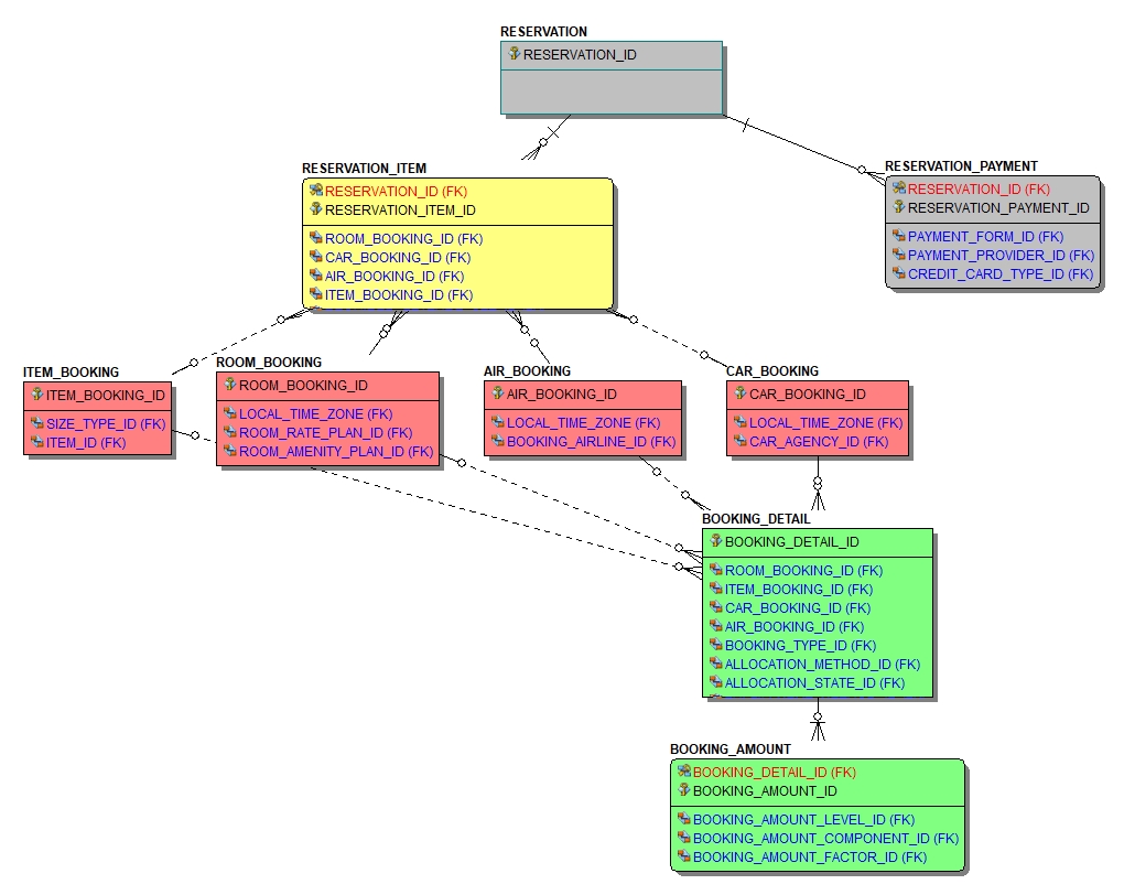
Let’s work through the logical and physical modeling process using a subset of our travel industry reservation model.   Here is the entity relationship diagram for the model:

A travel reservation is a variant of a standard sales order.  In the above model, colors are used to reflect the various levels of granularity within this model.  

• Grey – Reflects the itinerary or sales order level.  Your travel agency reservation confirmation number would be at this level.  
• Yellow – A reservation can be made up of multiple items.  For example, you may have booked a flight, hotel and car rental under the same travel agency reservation.   Like a sales order item, we carry the common attributes for each reservation item at this level of granularity.
• Red – Reservation items are bookings with different travel providers.  You booked your flight with United, your hotel with Marriot and your car rental with Avis.  Here we carry the attributes specific to the type of travel provider.    
• Green – Each booking (air, hotel or car) has fulfillment details associated with it.  In addition, there are attributes reflecting pricing details like rate, taxes, and fees.  

⇒ Semantic Model Example using our Travel Reservation Star Schema

As we design our semantic layer, we identify the levels of granularity we want to present to our business users and the associated measures we want to incorporate at that grain.  We represent these requirements using fact tables at the associated grain.  In our example, we are declaring fact tables at the reservation, reservation payment, and reservation item levels.   We also identify the supporting dimensions, their dimensional type and whether they are conformed dimensions in this semantic model.      

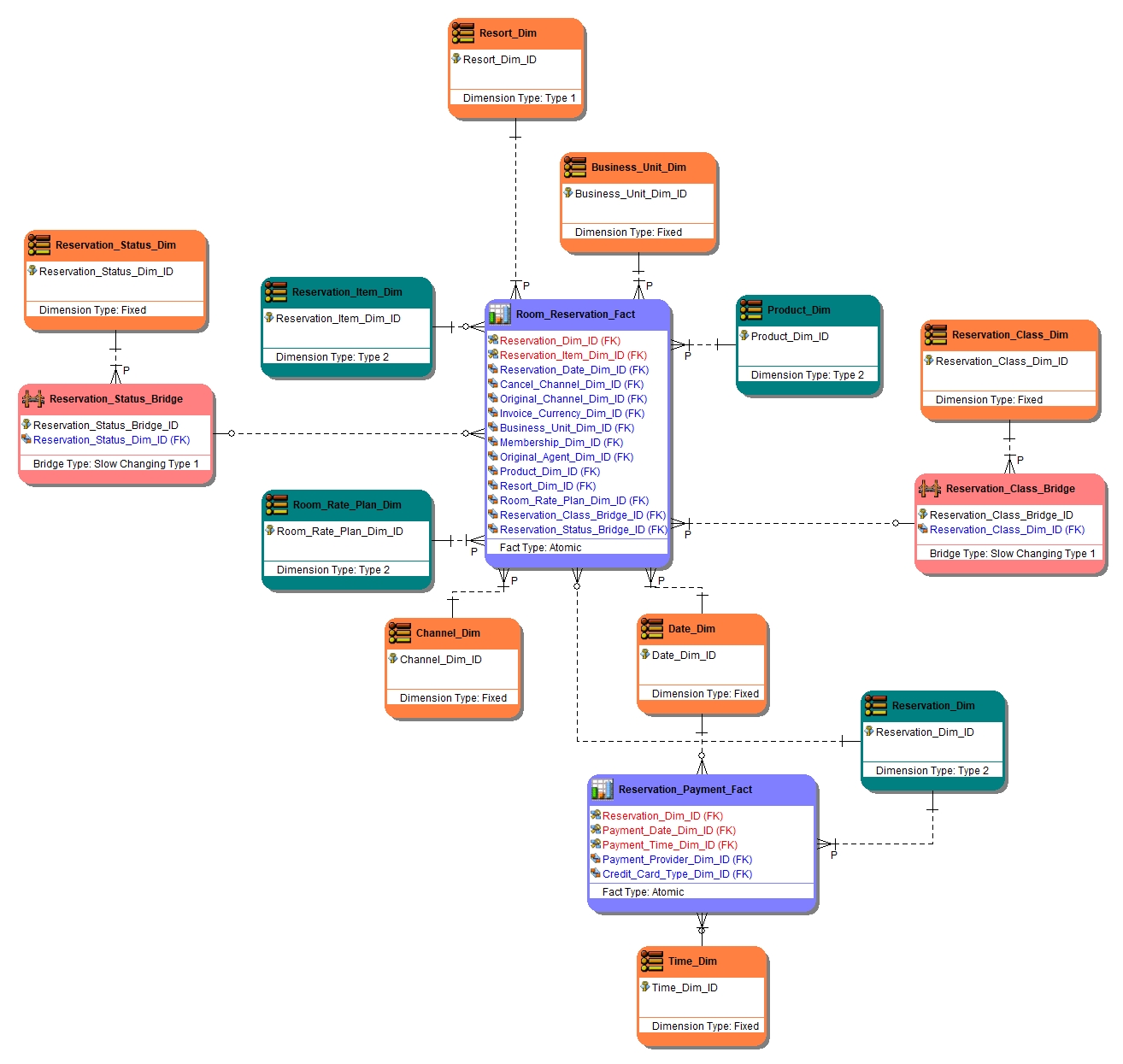
Let’s look at a subset of the star schema model we designed:

In the above model, colors are used to reflect the type of entity.   Let’s declare the grain of the two fact tables (shown in light blue):  

• Reservation_Payment_Fact – Payments are specific to a reservation as a whole, so the overall grain is reservation level.   The primary key is the reservation, payment date and payment time.  
• Room_Reservation_Fact – A room reservation is a specific booking type within a reservation item, so the overall grain is reservation item level.  The primary key is reservation and reservation item.

⇒ Physical Model Example for Reservation_Payment_Fact

Now let’s go through our physical modeling rules we discussed in “Creating the Physical Schema” above.

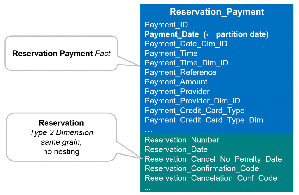
• What is the fact table grain? - The Reservation_Payment_Fact table is at reservation level.  
• How will the fact table be date partitioned? - It will be partitioned based on payment date (Payment_Dim_ID).  
• Are there type 2 dimension tables that are at the same grain as the fact table? – Yes, Reservation_Dim should be moved into the fact table.
• Are there large type 1 dimensions that might not efficiently join to the fact table? – No, Date_Dim and Time_Dim are small dimensions of static values.  While the fact that they contain static values would make them easy to move into the fact table, they are also conforming dimensions making our preference to leave them as separate tables until performance issues dictate a different approach.  

We end up with the following physical BigQuery table:

⇒ Physical Model Example for Room_Reservation_Fact

Using our physical modeling rules we discussed in “Creating the Physical Schema” above.

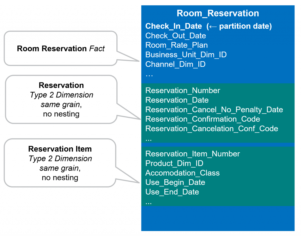
• What is the fact table grain? - The Room_Reservation_Fact table is at the reservation item level.  
• How will the fact table be date partitioned? - It will be partitioned based on reservation date (Reservation_Date_Dim_ID).  
• Are there type 2 dimension tables that are at the same grain as the fact table? – Yes, Reservation_Item_Dim should be moved into the fact table.    
• Are there large type 1 dimensions that might not efficiently join to the fact table? – No, Business_Unit_Dim and Channel_Dim are very small dimensions of static values.  Resort_Dim is a larger dimension, but it is a conforming dimension that we would leave as a separate table until performance issues dictate a different approach.   The two bridge tables Reservation_Status_Bridge and Reservation_Class_Bridge, each reference a single row in their associated dimensions.  We need these to stay as separate tables so that any change in the status of classification becomes immediately effective (type 1 point in time).
• Are there large type 2 dimensions that might not efficiently join to the fact table? – Yes, Reservation_Dim is at the reservation level and therefore can be moved into the fact table without any requirement for nested/repeating attributes.  Product_Dim is another conforming dimension that we would leave as a separate table until performance issues dictate a change.  Again, due to the star schema design, no requirement for nested/repeating attributes is needed.

We end up with the following physical table:

⇒ Additional Considerations

We try to keep conforming dimensions as separate tables as much as possible.   They are enterprise dimensions standardized across many subject areas.  They are typically enhanced (more attributes) over time as more and more subject areas use them.  As they are enhanced, every subject area using them should benefit, which will happen automatically if they remain as separate tables.

With BigQuery’s support for nested and repeating structures, we could have physically modeled this as a single nested table at the reservation grain, with nested structures for reservation item, room booking, booking detail and booking amount.  Essentially, you are just implementing your operational model as a single nested table and you will end up with nesting within nesting due to the relational nature of the original data model.   For this type of data, we find this nested/repeating structure more difficult to use for the business end user, and less compatible with many legacy BI tools implemented in your enterprise.  While we certainly implement BigQuery’s support for nested and repeating structures for other types of data structures (for example unstructured or XML based), in a Teradata conversion scenario, the dominant source data structures will be relational.   Therefore, we like the use the star schema fact table based approach.

⇒ Wrap-up, what’s next

In this third article of the series, we explored the details of how to design your data warehouse for Google Cloud BigQuery.  Starting with a semantic logical model, we discussed logical data modeling techniques using a star schema.  We then discussed how to apply a consistent set of physical modeling rules to the star schema in order to create a well performing physical schema for BigQuery.   Finally, we used a specific subject area example (travel reservations) to further explain the techniques we use.  

In the next (fourth) article of the series, we will start to discuss the data integration approaches that will be necessary to load the actual data warehouse.  We will focus introduce the staging area and the typical data integration use cases that require it.